DSF (Dense Subgraph Finder) 1.0 manual
1. What is Dense Subgraph Finder?
2. Installation
3. DSF usage
3.1. Basic options
3.2. Advanced options
3.3. Examples
3.4. Output files
4. GRAPH file format
5. Feedback and bug reports
5.1. Citation
1. What is Dense Subgraph Finder?
Problem of finding corrupted cliques is formulated as follows:
to find minimal number of edge additions and removals to convert graph into a set of cliques.
Search for corrupted cliques (or dense subgraphs) of some graph is a very common problem arising in bioinformatics
(e.g., co-expression of genes) and studies of social interactions (e.g., recommendation services).
DSF tool takes as an input indirected graph in GRAPH format and
outputs decomposition where the identical ids are assigned for vertices from the same dense subgraph.
Density of subgraph on N vertices and M edges is computed as ratio of M to maximal possible number of edges (N * (N - 1) / 2) and
can be tuned by user.
2. Installation
DSF comes as a part of IgRepertoireConstructor package.
See IgRepertoireConstructor manual for installation instructions.
Please verify your DSF installation prior to initiate the DSF:
./dense_subgraph_finder.py --test
If the installation is successful, you will find the following information at the end of the log:
  Thank you for using Dense Subgraph Finder!
  Log was written to <dsf_installation_dir>/dsf_test/dense_subgraph_finder.log
3. DSF usage
DSF takes as an input indirected (weighted or unweighted) graph in GRAPH format and
constructs dense subgraph decomposition.
To run DSF, type:
./dense_subgraph_finder.py [options] -g <input.graph> -o <output_dir>
3.1. Basic options
-g <input.graph>
indirected graph in GRAPH format (required).
-o / --output <output_dir>
output directory (required).
-t/--threads <int>
The number of parallel threads. The default value is 16.
--test
Running on the toy test dataset. Command line corresponding to the test run is equivalent to the following:
./dense_subgraph_finder.py -g test_dataset/test.graph -o dsf_test
--help
Printing help.
3.2. Advanced options
-f / --min-fillin <float>
Expected minimal edge fill-in of the constructed dense subgraphs.
Default value is 0.6.
-s / --min-size <int>
Minimal size of vertices in connected components of input graph where dense subgraphs will be computed.
Connected components which size do not exceed min-size will be decomposed trivially (all vertices are in the same dense subgraph).
Default value is 5.
-n / --min-snode-size <int>
Minimum node weight that is required to consider node heavy.
DSF algorithm does not glue two heavy vertices into the same dense subgraph.
If graph is edge weighted only, vertex weights are equal to 1.
Default value is 5.
--save-aux-files
Saving dense subgraph decompositions for connected components.
3.3. Examples
To construct dense subgraph decomposition for graph input.graph with
minimal edge fill-in value 0.9, type:
./dense_subgraph_finder.py -g input.graph -f 0.9 -o dsf_test
3.4. Output files
DSF creates working directory (which name was specified using option -o)
and outputs the following files there:
- dense_subgraphs.txt — dense subgraph decomposition in TXT format,
i-th line of dense_subgraphs.txt file corresponds to i-th vertex and contains index (zero-based) of dense subgraph contaning this vertex.
-
dense_subgraph_finder.log — full log of DSF.
DSF takes undirected edge weighted or unweigthed graphs in
GRAPH format.
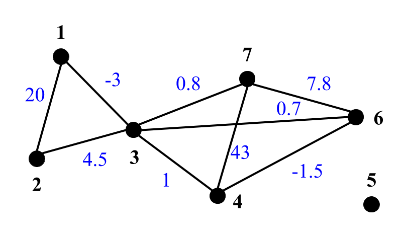
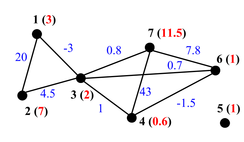
Below are examples representation of unweigthed (left) and edge weighted (middle) and edge & vertex weighted (right) graphs in GRAPH format:

|
|

|
|

|
7 9
2 3
1 3
1 2 4 6 7
3 6 7
3 4 7
3 4 6
|
|
7 9 001
2 20 3 -3
1 20 3 4.5
1 -3 2 4.5 4 1
6 0.7 7 0.8
3 1 6 -1.5 7 43
3 0.7 4 -1.5 7 7.8
3 0.8 4 43 6 7.8
|
|
7 9 011
3 2 20 3 -3
7 1 20 3 4.5
2 1 -3 2 4.5 4 1 6 0.7 7 0.8
0.6 3 1 6 -1.5 7 43
1
1 3 0.7 4 -1.5 7 7.8
11.5 3 0.8 4 43 6 7.8
|
|
The first line shows number of vertices (7) and number of edges (9).
Each of the next lines contains vertex neighbours.
E.g., the second line notes that vertex 1 is connected with vertices 2 and 3.
|
|
The first line shows number of vertices (7), number of edges (9) and description 001 that denotes edge weighted graph.
Each of the next lines contains vertex neighbours and weights of corresponding edges (highlighted in blue) for graph vertices.
E.g., the second line notes that vertex 1 is connected with vertex 2 by edge of weigth 20 and
vertex 3 by the edge of weigth -3.
|
|
The first line shows number of vertices (7), number of edges (9) and description 011 that denotes edge & vertex weighted graph.
Each of the next lines contains vertex weight (highlighed in red), its neighbours and weights of corresponding edges (highlighted in blue).
E.g., the second line notes that vertex 1 of weight 3 is connected with vertex 2 by edge of weigth 20 and
vertex 3 by the edge of weigth -3.
|
Please note that numeration of vertices is 1-based.
Isolated vertices (vertices without neighbours) are denoted by empty lines for unweighted and edge weighted graphs.
5. Feedback and bug reports
Your comments, bug reports, and suggestions are very welcome.
They will help us to further improve DSF.
If you have any trouble running DSF, please send us the log file from the output directory.
Address for communications: igtools_support@googlegroups.com.
5.1. Citation
If you use DSF in your research, please refer to
Safonova et al., 2015.


